Machine Learning Applied to Stock Market Prediction: A Comparison between LSTM and ESN
Published:
I have been working with various neural networks for a while and always find recurrent neural network (RNN) very special. Whenever, there is a dependency with previous data points, then these networks shines out. Time-series problem especially fits here for e.g. predicting the weather pattern or stock market. In the past, I have done work to compare various RNNs for such tasks and my work concluded that ESN works quite well compared to simple deep neural network and some RNNs like LSTM or GRU (paper-1, paper-2 and paper-3) (of course this statement vary with the domain). Those works were done mostly with the scientific data for turbulent flow for thermal plumes, which has significant effects on weather (Wikipedia). Now, I was curious to see how these network can work for practical purpose.
Use case
My use-case is focused on stock market price prediction, especially the opening price for a given stock. I haven’t focused too much on the hyperparameter tuning, rather aimed towards building the basic model and comparing some results. Unlike the scientific work, where my network has to predict autonomously provided an initial data, here we have the luxury to get input continuously i.e. by the end of the day we will have all the inputs so that we can guess what will be the opening price tomorrow.
About the RNNs
RNN are suitable, especially when there is a sequence and each value in the sequence is dependent on the previous values. For e.g. time-series like temperature during the day, words in a sentence etc. On the other hand, simple feed forward neural networks are suited when data points or input variables are independent (more or less). For more exact details, this article can be useful. In the following, we will focus on 2 different variants of RNNs.
Long Short-Term Memory (LSTM) and Gated Recurrent Units (GRU)
Plain RNNs are prone to the problem of vanishing gradient, therefore LSTM and GRU algorithms have specific gate which restrict the information flow from the past. This is a super useful blog to understand the working of LSTM. GRU is slightly differing but once you know LSTM then it’s easy to understand, for instance see this towardsdatascience article.
ESN
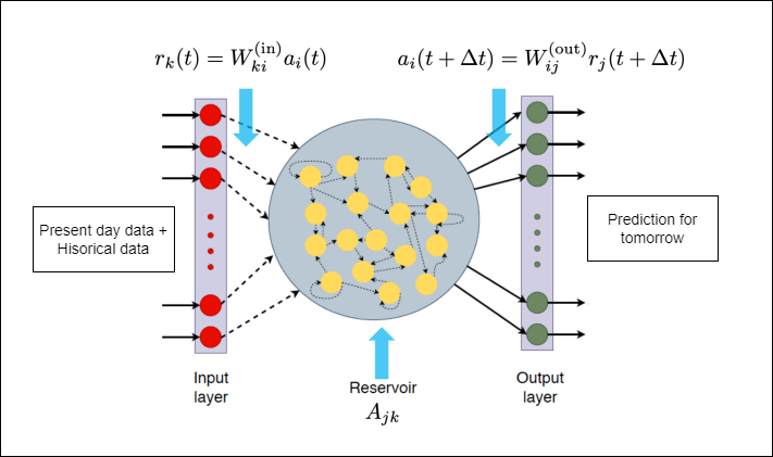
ESN belongs to the Reservoir Computing Model (RCM) framework, which was established in early 2000s. There are few blogs (like this and this) which already explain it in details, while this answer explains the intuition behind it. Here, I briefly explain so that it make sense when we do the implementation. Similar to the other RNNs, the ESN has an input and an output layer, in our case the input is composed of 4 features on given day, and we look back for 7 days as history point. It means, our input is of size 28 (represented as single 1D array in the notebook) similar to LSTM (represented by 7×4 2D array).
Instead of several hidden layers, the input layer is connected to a state vector in the reservoir with the randomly initialized N×1 weight matrix $W_{in}$ and N. While matrices $W_{in}$ and A remain fixed in the training procedure, the output 1×N weight matrix, which is defined via $a_{out}(t)$ updated by a standard optimization procedure. In addition to the training without expensive back-propagation in a multi-layered LSTM networks, reservoir computing methods thus provide a high-dimensional dynamical system Details with actual equations can be found in this paper.

Experiments
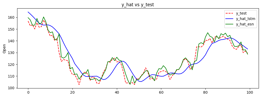
For the given use case, I experimented with the stock market data and tried LSTM and ESN to make a high-level, quick comparison. This example is illustrated using this notebook which you can try out by yourself. As mentioned, both the model are used as it is without focusing on hyperparameter tuning, so there is a lot of scope to improve this. But, that can also be a fair comparison, as I started randomly. The data preprocessing part is similar in both the network, i.e. arranging the data with previous history point. While the setting up model and training was easy for ESN. ESN took 219 ms to train, while LSTM took 17.6 s, so a completely different of order of magnitude. This was expected because ESN doesn’t have the back-propagation as explained in the previous section. When we compare the results, then the results from the former definitely looks much better.

It is also interesting to note that trend and peaks are better captured by the ESN even with very sparse connectivity of the neurons within the reservoir, that’s pretty impressive! The shift of values between prediction from ESN and GT is lower than prediction from LSTM. This was a rather simple problem (for capturing trend, not for having lowest error), and it is obvious that ESN has potential which deserves a proper attention. In our scientific work, we had 10s of input and output variables in the dynamical system, and ESN was certainly giving better results.
Reach out to me on Instagram for a faster reply! 
